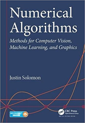
Numerical Algorithms Methods for Computer Vision Machine Learning and Graphics 1st Solomon Solution Manual
$55.00 Original price was: $55.00.$29.99Current price is: $29.99.
Numerical Algorithms Methods for Computer Vision Machine Learning and Graphics 1st Solomon Solution Manual
Numerical Algorithms Methods for Computer Vision Machine Learning and Graphics 1st Solomon Solution Manual
Product details:
- ISBN-10 : 1482251884
- ISBN-13 : 978-1482251883
- Author: Justin Solomon
Numerical Algorithms: Methods for Computer Vision, Machine Learning, and Graphics presents a new approach to numerical analysis for modern computer scientists. Using examples from a broad base of computational tasks, including data processing, computational photography, and animation, the textbook introduces numerical modeling and algorithmic design from a practical standpoint and provides insight into the theoretical tools needed to support these skills.
Table contents:
- CHAPTER 1 Mathematics Review
- 1.1 PRELIMINARIES: NUMBERS AND SETS
- 1.2 VECTOR SPACES
- 1.2.1 Defining Vector Spaces
- Definition 1.1
- Example 1.1
- Figure 1.1 (a) Vectors (b) their span is the plane ℝ2; (c) because is a linear combination of and
- Example 1.2
- 1.2.2 Span, Linear Independence, and Bases
- Definition 1.2
- Example 1.3
- Example 1.4
- Definition 1.3
- Definition 1.4
- Example 1.5
- Example 1.6
- 1.2.3 Our Focus: ℝn
- Definition 1.5
- Example 1.7
- Definition 1.6
- Aside 1.1.
- 1.3 LINEARITY
- Definition 1.7
- Example 1.8
- Example 1.9
- Example 1.10
- 1.3.1 Matrices
- Example 1.11
- Example 1.12
- Example 1.13
- Example 1.14
- 1.3.2 Scalars, Vectors, and Matrices
- Definition 1.8
- Example 1.15
- Example 1.16
- Figure 1.2 Two implementations of matrix-vector multiplication with different loop ordering.
- 1.3.3 Matrix Storage and Multiplication Methods
- Figure 1.3 Two possible ways to store (a) a matrix in memory: (b) row-major ordering and (c) column-major ordering.
- 1.3.4 Model Problem:
- Definition 1.9
- 1.4 NON-LINEARITY: DIFFERENTIAL CALCULUS
- Figure 1.4 The closer we zoom into f(x) = x3 + x2 − 8x + 4, the more it looks like a line.
- 1.4.1 Differentiation in One Variable
- Figure 1.5 Big-O notation; in the ε neighborhood of the origin, f(x) is dominated by Cg(x); outside this neighborhood, Cg(x) can dip back down.
- Definition 1.10
- 1.4.2 Differentiation in Multiple Variables
- Definition 1.11
- Figure 1.6 We can visualize a function f(x1, x2) as a three-dimensional graph; then is the direction on the (x1, x2) plane corresponding to the steepest ascent of f. Alternatively, we can think of f(x1, x2) as the brightness at (x1, x2) (dark indicates a low value of f), in which case ▿f points perpendicular to level sets in the direction where f is increasing and the image gets lighter.
- Example 1.17
- Example 1.18
- Example 1.19
- Example 1.20
- Definition 1.12
- Example 1.21
- Example 1.22
- 1.4.3 Optimization
- Example 1.23
- Example 1.24
- Figure 1.7 Three rectangles with the same perimeter 2w + 2h but unequal areas wh; the square on the right with w = h maximizes wh over all possible choices with prescribed 2w + 2h = 1.
- Example 1.25
- Figure 1.8 (a) An equality-constrained optimization. Without constraints, is minimized at the star; solid lines show isocontours for increasing c. Minimizing subject to forces to be on the dashed curve, (b) The point is suboptimal since moving in the direction decreases while maintaining (c) The point is optimal since decreasing f from would require moving in the −▿f direction, which is perpendicular to the curve
- Theorem 1.1
- Example 1.26
- Example 1.27
- 1.5 EXERCISES
- CHAPTER 2 Numerics and Error Analysis
- 2.1 STORING NUMBERS WITH FRACTIONAL PARTS
- 2.1.1 Fixed-Point Representations
- 2.1.2 Floating-Point Representations
- Figure 2.1 The values from Example 2.1 plotted on a number line; typical for floating-point number systems, they are unevenly spaced between the minimum (0.5) and the maximum (3.5).
- Example 2.1
- 2.1.3 More Exotic Options
- 2.2 UNDERSTANDING ERROR
- Example 2.2
- 2.2.1 Classifying Error
- Definition 2.1
- Definition 2.2
- Example 2.3
- Example 2.4
- Figure 2.2 Values of f(x) from Example 2.5, computed using IEEE floating-point arithmetic.
- Example 2.5
- Definition 2.3
- Example 2.6
- Example 2.7
- 2.2.2 Conditioning, Stability, and Accuracy
- Example 2.8
- Definition 2.4
- Example 2.9
- Example 2.10
- 2.3 PRACTICAL ASPECTS
- 2.3.1 Computing Vector Norms
- Figure 2.3 (a) A simplistic method for summing the elements of a vector (b) the Kahan summation algorithm.
- 2.3.2 Larger-Scale Example: Summation
- 2.4 EXERCISES
- Figure 2.4 z-fighting, for Exercise 2.6; the overlap region is zoomed on the right.
- II Linear Algebra
- CHAPTER 3 Linear Systems and the LU Decomposition
- 3.1 SOLVABILITY OF LINEAR SYSTEMS
- 3.2 AD-HOC SOLUTION STRATEGIES
- 3.3 ENCODING ROW OPERATIONS
- 3.3.1 Permutation
- Example 3.1
- 3.3.2 Row Scaling
- 3.3.3 Elimination
- Example 3.2
- Example 3.3
- 3.4 GAUSSIAN ELIMINATION
- 3.4.1 Forward-Substitution
- Figure 3.1 Forward-substitution without pivoting; see §3.4.3 for pivoting options.
- 3.4.2 Back-Substitution
- 3.4.3 Analysis of Gaussian Elimination
- Figure 3.2 Back-substitution for solving upper-triangular systems; this implementation returns the solution to the system without modifying U.
- Example 3.4
- 3.5 LU FACTORIZATION
- 3.5.1 Constructing the Factorization
- Proposition 3.1
- 3.5.2 Using the Factorization
- 3.5.3 Implementing LU
- 3.6 EXERCISES
- Figure 3.3 Pseudocode for computing the LU factorization of A ∈ ℝnxn, stored in the compact n × n format described in §3.5.3. This algorithm will fail if pivoting is needed.
- CHAPTER 4 Designing and Analyzing Linear Systems
- 4.1 SOLUTION OF SQUARE SYSTEMS
- Figure 4.1 (a) The input for regression, a set of (x(k), y(k)) pairs; (b) a set of basis functions {f1, f2, f3, f4}; (c) the output of regression, a set of coefficients c1, …, c4 such that the linear combination goes through the data points.
- 4.1.1 Regression
- Example 4.1
- Example 4.2
- Example 4.3
- Figure 4.2 Drawbacks of fitting function values exactly: (a) noisy data might be better represented by a simple function rather than a complex curve that touches every data point and (b) the basis functions might not be tuned to the function being sampled. In (b), we fit a polynomial of degree eight to nine samples from f(x) = |x| but would have been more successful using a basis of line segments.
- Example 4.4
- 4.1.2 Least-Squares
- Theorem 4.1
- 4.1.3 Tikhonov Regularization
- Example 4.5
- 4.1.4 Image Alignment
- Figure 4.3 (a) The image alignment problem attempts to find the parameters A and of a transformation from one image of a scene to another using labeled keypoints on the first image paired with points on the second. As an example, keypoints marked in white on the two images in (b) are used to create (c) the aligned image.
- Figure 4.4 Suppose rather than taking (a) the sharp image, we accidentally take (b) a blurry photo; then, deconvolution can be used to recover (c) a sharp approximation of the original image. The difference between (a) and (c) is shown in (d); only high-frequency detail is different between the two images.
- 4.1.5 Deconvolution
- Figure 4.5 (a) An example of a triangle mesh, the typical structure used to represent three-dimensional shapes in computer graphics, (b) In mesh parameterization, we seek a map from a three-dimensional mesh (left) to the two-dimensional image plane (right); the right-hand side shown here was computed using the method suggested in §4.1.6. (c) The harmonic condition is that the position of vertex is the average of the positions of its neighbors w1, …, w5.
- 4.1.6 Harmonic Parameterization
- 4.2 SPECIAL PROPERTIES OF LINEAR SYSTEMS
- 4.2.1 Positive Definite Matrices and the Cholesky Factorization
- Definition 4.1
- Proposition 4.1
- Aside 4.1
- Example 4.6
- Example 4.7
People also search:
numerical algorithms methods for computer vision machine learning and graphics
|
numerical methods for machine learning
computer vision algorithms and applications solution manual pdf
|
You may also like…
Solution Manual
Solution Manual for Numerical Methods for Engineers, 8th Edition By Steven Chapra Raymond Canale
Solution Manual
Solution Manual for Computer Vision: A Modern Approach, 2/E 2nd Edition : 013608592X
Solution Manual
Solution Manual
Solution Manual


